1 import tensorflow as tf 导入tensorflow
Tensorflow学习代码
链接:https://pan.baidu.com/s/1LJM8_QoT-Z88VYwZhSonFw
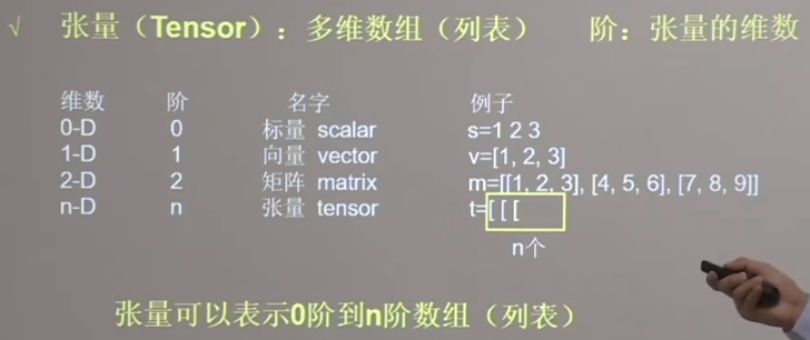
Tensor数据 1 2 3 list np.array科学计算库 tf.Tensor支持连续求导
创建tensor tf.constant([1,5], dtype=tf.int64)创建一个tensor
tf.convert_to_tensor(np, dtype=tf.int64)可以将numpy数据转换为tensor
1 2 3 4 5 6 7 8 tf.constant([1,5], dtype=tf.int64)创建一个张量 tf.convert_to_tensor(np, dtype=tf.int64)将numpy数据转换为tensor tf.zeros(维度)创建全为0的tensor tf.ones(维度)创建全为0的tensor tf.fill(维度, 指定值)创建全为指定值的tensor tf.random.normal(维度, mean=, stddev=)创建指定维度的正态分布随机数 tf.random.truncated_normal(维度, mean=, stddev=)创建指定维度的正态分布随机数,其中所有数值都在(μ-2σ,μ+2σ)范围内 tf.uniform(维度,minval=,maxval)生成指定维度均匀分布的随机数
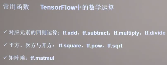
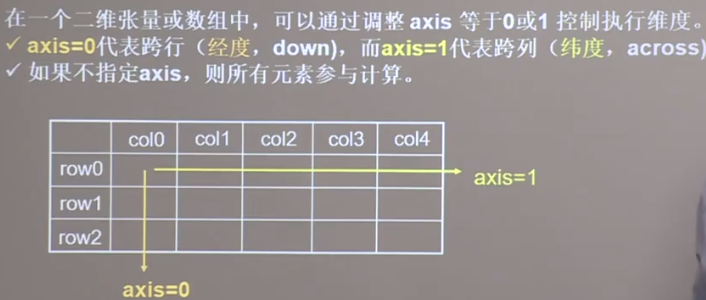
常用函数 1 2 3 4 5 6 7 tf.cast(tf, dtype=)强制转换tensor中的数据类型 tf.reduce_min(tf)计算最小值 tf.reduce_max(tf)计算最大值 tf.reduce_mean(tf, axis=)计算指定经度的平均值(不指定axis则对所有数据进行操作) tf.reduce_sum(tf, axis=)计算指定经度的和(不指定axis则对所有数据进行操作) tf.Variable(tf)将变量标记为可训练,变量在反向传播中记录梯度信息 其他数学运算如下图
维度相同的tensor才能进行数学运算
axis
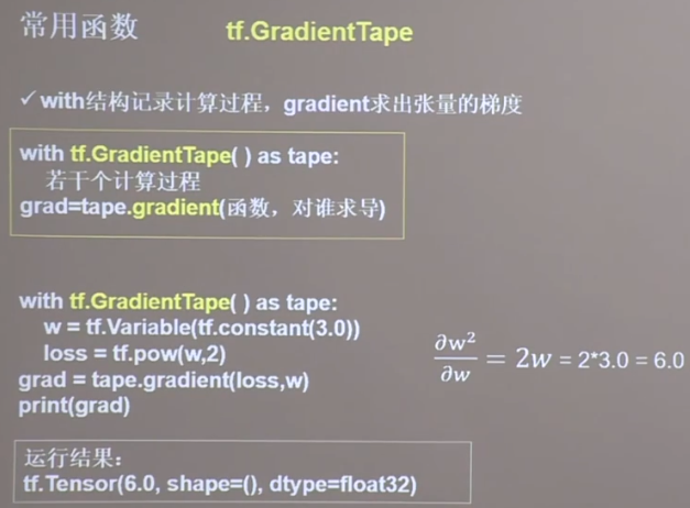
1 2 3 4 5 6 7 8 9 tf.data.Dataset.from_tensor_slices((features, labels))将数据与标签配对 tf.GradientTape()实现loss对参数w的求导计算,如图(需要variable类型) enumerate(列表/元组/字符串)枚举每一个元素并组合为索引元素(为python自带函数) tf.one_hot(tf, depth=几分类) tf.nn.softmax(tf)将数据转换为总和为一且每一项大于0的数据,常用于逻辑回归 tf.assign_sub(w自减内容),赋值操作,更新参数并返回(需要variable类型) tf.argmax(tf,axis=)返回指定轴最大值索引 tf.where(条件语句, a, b)若为真返回a对应位置元素,若为假返回b对应位置元素 np.random.RandomState.rand(维度)
独热码one-hot
获取数据集 1 2 3 from sklearn.datasets import load_iris x_data=datasets.load_iris().data获取特征值 y_data=datasets.load_iris().target获取标签
numpy常用函数 1 2 np.random.RandomState.rand(维度) np.vstack(数组1, 数组2)两个数组垂直方向叠加
随机数种子
1 2 3 np.mgrid[] } np.ravel() }联合使用可以创建网格坐标点,如下图 np.c_[] }
神经网络实现 指数衰减学习率 1 2 3 4 5 6 7 8 9 10 11 12 13 14 15 16 17 import tensorflow as tfw = tf.Variable(tf.constant(5 , dtype=tf.float32)) epoch = 40 LR_BASE = 0.2 LR_DECAY = 0.99 LR_STEP = 1 for epoch in range(epoch): lr = LR_BASE * LR_DECAY ** (epoch / LR_STEP) with tf.GradientTape() as tape: loss = tf.square(w + 1 ) grads = tape.gradient(loss, w) w.assign_sub(lr * grads) print("After %s epoch,w is %f,loss is %f,lr is %f" % (epoch, w.numpy(), loss, lr))
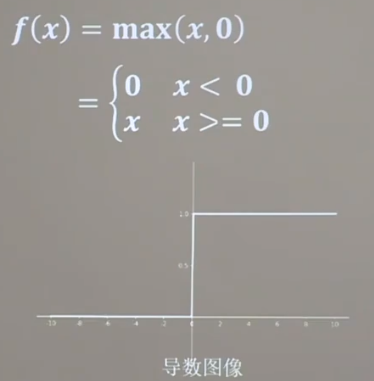
激活函数 relu函数 初学者首选
均值非0导致收敛变慢,同时可能存在dead_relu问题,即激活函数输出为0,反向传播得到梯度为0,参数无法更新,神经元死亡
改进方法:随机初始化,减小学习率
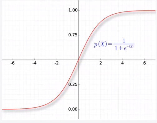
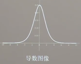
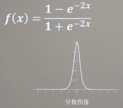
sigmoid函数
反向传播需要多个导数项相乘,sigmoid函数导数都在0~0.25之间,导致梯度消失,参数无法继续更新;同时,存在幂运算导致计算量偏大
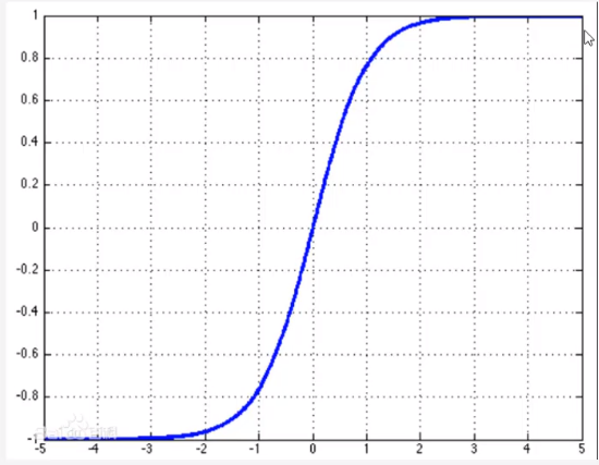
tanh函数
与sigmoid函数相同,具有梯度消失和幂运算问题
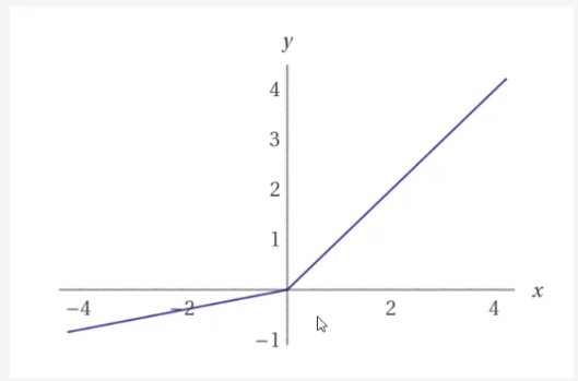
leak relu函数 负值影响较小
效果比relu更好,但一般还是选择relu
代码实现 1 2 3 4 5 6 7 8 9 10 11 12 13 14 15 16 17 18 19 20 21 import tensorflow as tfimport pandas as pdimport numpy as npimport matplotlib.pyplot as plt%matplot-inline data=pd.read_csv("./datasets.csv" ) x = data.iloc[:,1 :-1 ] y = data.iloc[:, -1 ] model = tf.keras.Sequential([tf.keras.layers.Dense(10 , input_shape=(3 ,), activation='relu' ), tf.keras.layers.Dense(1 )] ) model.summary() model.compile(optimizer='adam' , loss='mse' ) model.fit(x,y,epochs=1000 ) model.predict(Test)
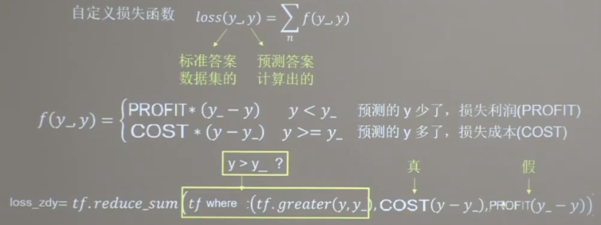
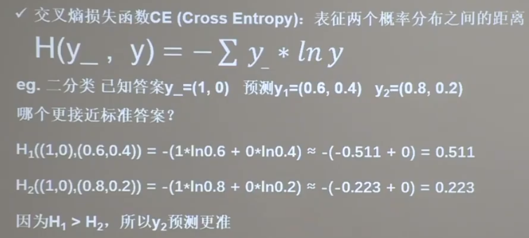
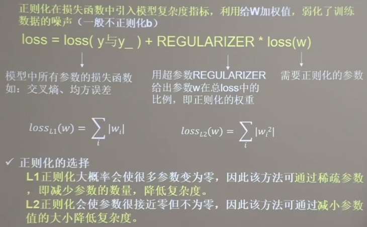
损失函数 1 2 3 4 tf.reduce_mean(tf)计算均方差 tf.losses.categorical_crossentropy(y_, y)计算交叉熵 tf.nn.softmax_cross_entropy_with_logits(y_, y)将softmax与交叉熵结合,用于多分类问题 自定义损失函数,如下图
正则化
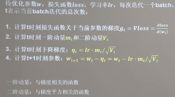
神经网络参数优化器
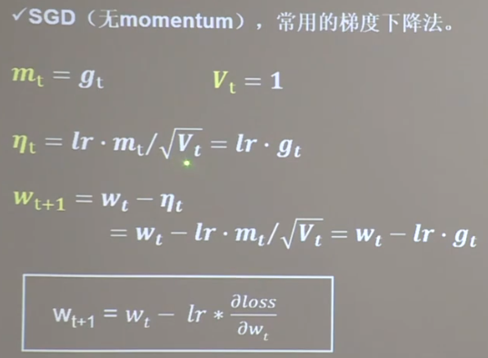
SGD
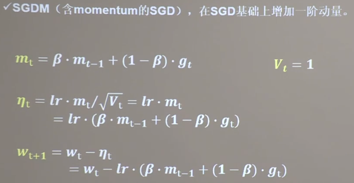
SGDM
m_t-1表示上一时刻的动量
实现代码(部分)
1 2 3 4 5 6 7 m_w, m_b = 0 , 0 beta = 0.9 m_w = beta * m_w + (1 - beta) * grads[0 ] m_b = beta * m_b + (1 - beta) * grads[1 ] w1.assign_sub(lr * m_w) b1.assign_sub(lr * m_b)
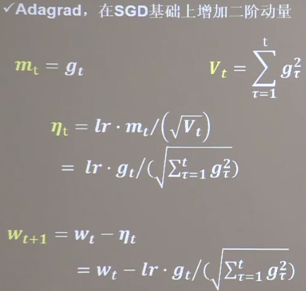
Adagrad
实现代码(部分)
1 2 3 4 5 6 v_w, v_b = 0 , 0 v_w += tf.square(grads[0 ]) v_b += tf.square(grads[1 ]) w1.assign_sub(lr * grads[0 ] / tf.sqrt(v_w)) b1.assign_sub(lr * grads[1 ] / tf.sqrt(v_b))
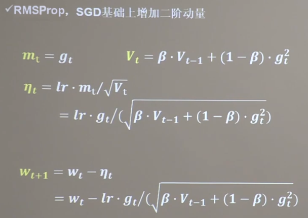
RMSProp
代码实现(部分)
1 2 3 4 5 6 7 v_w, v_b = 0 , 0 beta = 0.9 v_w = beta * v_w + (1 - beta) * tf.square(grads[0 ]) v_b = beta * v_b + (1 - beta) * tf.square(grads[1 ]) w1.assign_sub(lr * grads[0 ] / tf.sqrt(v_w)) b1.assign_sub(lr * grads[1 ] / tf.sqrt(v_b))
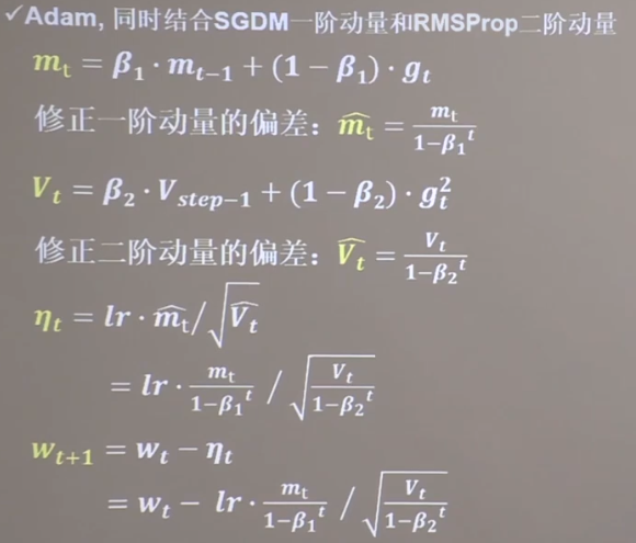
Adam
代码实现(部分)
1 2 3 4 5 6 7 8 9 10 11 12 13 14 15 16 17 18 m_w, m_b = 0 , 0 v_w, v_b = 0 , 0 beta1, beta2 = 0.9 , 0.999 delta_w, delta_b = 0 , 0 global_step = 0 m_w = beta1 * m_w + (1 - beta1) * grads[0 ] m_b = beta1 * m_b + (1 - beta1) * grads[1 ] v_w = beta2 * v_w + (1 - beta2) * tf.square(grads[0 ]) v_b = beta2 * v_b + (1 - beta2) * tf.square(grads[1 ]) m_w_correction = m_w / (1 - tf.pow(beta1, int(global_step))) m_b_correction = m_b / (1 - tf.pow(beta1, int(global_step))) v_w_correction = v_w / (1 - tf.pow(beta2, int(global_step))) v_b_correction = v_b / (1 - tf.pow(beta2, int(global_step))) w1.assign_sub(lr * m_w_correction / tf.sqrt(v_w_correction)) b1.assign_sub(lr * m_b_correction / tf.sqrt(v_b_correction))
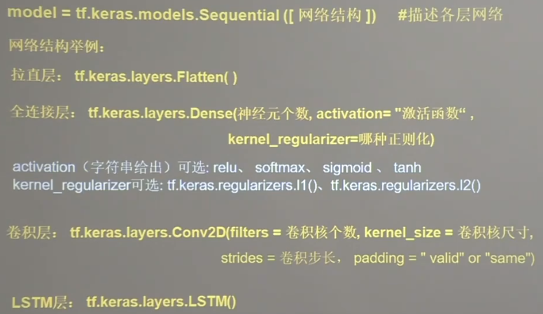
全连接网络 六步法搭建神经网络
import
train, test
model=tf.keras.models.Sequential
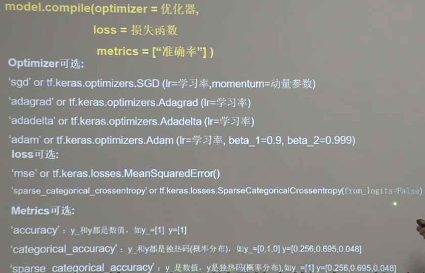
model.compile
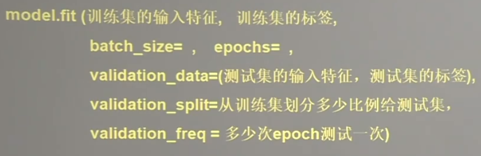
model.fit
model.summary
方法描述 model=tf.keras.models.Sequential 包含了各种网络结构:拉直层、全连接层、卷积层、LSTM层
compile
fit 使用时validation_data和validation_split二选一
summary 在终端输出训练结果
代码实现 1 2 3 4 5 6 7 8 9 10 11 12 13 14 15 16 17 18 19 20 21 22 23 24 25 import tensorflow as tffrom sklearn import datasetsimport numpy as npx_train = datasets.load_iris().data y_train = datasets.load_iris().target np.random.seed(116 ) np.random.shuffle(x_train) np.random.seed(116 ) np.random.shuffle(y_train) tf.random.set_seed(116 ) model = tf.keras.models.Sequential([ tf.keras.layers.Dense(3 , activation='softmax' , kernel_regularizer=tf.keras.regularizers.l2()) ]) model.compile(optimizer=tf.keras.optimizers.SGD(lr=0.1 ), loss=tf.keras.losses.SparseCategoricalCrossentropy(from_logits=False ), metrics=['sparse_categorical_accuracy' ]) model.fit(x_train, y_train, batch_size=32 , epochs=500 , validation_split=0.2 , validation_freq=20 ) model.summary()
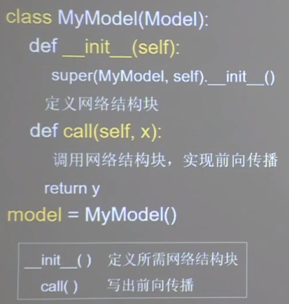
class MyModel(Model) model=MyModel 将之前的Sequential替换为自定义class继承Model类
代码实现 相比之下,导入模块增加了Dense和Model,然后自定义IrisModel类来创建神经网络结构
1 2 3 4 5 6 7 8 9 10 11 12 13 14 15 16 17 18 19 20 21 22 23 24 25 26 27 28 29 30 31 32 import tensorflow as tffrom tensorflow.keras.layers import Densefrom tensorflow.keras import Modelfrom sklearn import datasetsimport numpy as npx_train = datasets.load_iris().data y_train = datasets.load_iris().target np.random.seed(116 ) np.random.shuffle(x_train) np.random.seed(116 ) np.random.shuffle(y_train) tf.random.set_seed(116 ) class IrisModel (Model ): def __init__ (self ): super(IrisModel, self).__init__() self.d1 = Dense(3 , activation='softmax' , kernel_regularizer=tf.keras.regularizers.l2()) def call (self, x ): y = self.d1(x) return y model = IrisModel() model.compile(optimizer=tf.keras.optimizers.SGD(lr=0.1 ), loss=tf.keras.losses.SparseCategoricalCrossentropy(from_logits=False ), metrics=['sparse_categorical_accuracy' ]) model.fit(x_train, y_train, batch_size=32 , epochs=500 , validation_split=0.2 , validation_freq=20 ) model.summary()
mnist数据集
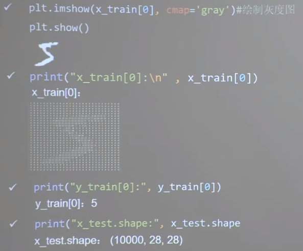
查看数据集 1 2 3 4 5 6 7 8 9 10 11 12 13 14 15 16 17 18 19 20 21 22 23 import tensorflow as tffrom matplotlib import pyplot as pltmnist = tf.keras.datasets.mnist (x_train, y_train), (x_test, y_test) = mnist.load_data() plt.imshow(x_train[0 ], cmap='gray' ) plt.show() print("x_train[0]:\n" , x_train[0 ]) print("y_train[0]:\n" , y_train[0 ]) print("x_train.shape:\n" , x_train.shape) print("y_train.shape:\n" , y_train.shape) print("x_test.shape:\n" , x_test.shape) print("y_test.shape:\n" , y_test.shape)
Sequential实现 1 2 3 4 5 6 7 8 9 10 11 12 13 14 15 16 17 18 19 import tensorflow as tfmnist = tf.keras.datasets.mnist (x_train, y_train), (x_test, y_test) = mnist.load_data() x_train, x_test = x_train / 255.0 , x_test / 255.0 model = tf.keras.models.Sequential([ tf.keras.layers.Flatten(), tf.keras.layers.Dense(128 , activation='relu' ), tf.keras.layers.Dense(10 , activation='softmax' ) ]) model.compile(optimizer='adam' , loss=tf.keras.losses.SparseCategoricalCrossentropy(from_logits=False ), metrics=['sparse_categorical_accuracy' ]) model.fit(x_train, y_train, batch_size=32 , epochs=5 , validation_data=(x_test, y_test), validation_freq=1 ) model.summary()
自定义class实现 1 2 3 4 5 6 7 8 9 10 11 12 13 14 15 16 17 18 19 20 21 22 23 24 25 26 27 28 29 30 31 import tensorflow as tffrom tensorflow.keras.layers import Dense, Flattenfrom tensorflow.keras import Modelmnist = tf.keras.datasets.mnist (x_train, y_train), (x_test, y_test) = mnist.load_data() x_train, x_test = x_train / 255.0 , x_test / 255.0 class MnistModel (Model ): def __init__ (self ): super(MnistModel, self).__init__() self.flatten = Flatten() self.d1 = Dense(128 , activation='relu' ) self.d2 = Dense(10 , activation='softmax' ) def call (self, x ): x = self.flatten(x) x = self.d1(x) y = self.d2(x) return y model = MnistModel() model.compile(optimizer='adam' , loss=tf.keras.losses.SparseCategoricalCrossentropy(from_logits=False ), metrics=['sparse_categorical_accuracy' ]) model.fit(x_train, y_train, batch_size=32 , epochs=5 , validation_data=(x_test, y_test), validation_freq=1 ) model.summary()
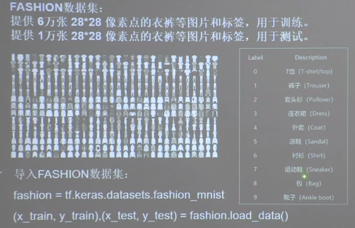
fashion数据集
Sequential实现 1 2 3 4 5 6 7 8 9 10 11 12 13 14 15 16 17 18 import tensorflow as tffashion = tf.keras.datasets.fashion_mnist (x_train, y_train),(x_test, y_test) = fashion.load_data() x_train, x_test = x_train / 255.0 , x_test / 255.0 model = tf.keras.models.Sequential([ tf.keras.layers.Flatten(), tf.keras.layers.Dense(128 , activation='relu' ), tf.keras.layers.Dense(10 , activation='softmax' ) ]) model.compile(optimizer='adam' , loss=tf.keras.losses.SparseCategoricalCrossentropy(from_logits=False ), metrics=['sparse_categorical_accuracy' ]) model.fit(x_train, y_train, batch_size=32 , epochs=5 , validation_data=(x_test, y_test), validation_freq=1 ) model.summary()
补充方法 自制数据集 实现代码(部分) 1 2 3 4 5 6 7 8 9 10 11 12 13 14 15 16 17 18 19 20 21 22 23 24 25 26 27 28 29 30 31 32 33 34 35 36 37 38 39 40 41 42 43 44 45 46 47 48 49 50 51 52 53 54 55 56 57 58 import tensorflow as tffrom PIL import Imageimport numpy as npimport ostrain_path = './mnist_image_label/mnist_train_jpg_60000/' train_txt = './mnist_image_label/mnist_train_jpg_60000.txt' x_train_savepath = './mnist_image_label/mnist_x_train.npy' y_train_savepath = './mnist_image_label/mnist_y_train.npy' test_path = './mnist_image_label/mnist_test_jpg_10000/' test_txt = './mnist_image_label/mnist_test_jpg_10000.txt' x_test_savepath = './mnist_image_label/mnist_x_test.npy' y_test_savepath = './mnist_image_label/mnist_y_test.npy' def generateds (path, txt ): f = open(txt, 'r' ) contents = f.readlines() f.close() x, y_ = [], [] for content in contents: value = content.split() img_path = path + value[0 ] img = Image.open(img_path) img = np.array(img.convert('L' )) img = img / 255. x.append(img) y_.append(value[1 ]) print('loading : ' + content) x = np.array(x) y_ = np.array(y_) y_ = y_.astype(np.int64) return x, y_ if os.path.exists(x_train_savepath) and os.path.exists(y_train_savepath) and os.path.exists( x_test_savepath) and os.path.exists(y_test_savepath): print('-------------Load Datasets-----------------' ) x_train_save = np.load(x_train_savepath) y_train = np.load(y_train_savepath) x_test_save = np.load(x_test_savepath) y_test = np.load(y_test_savepath) x_train = np.reshape(x_train_save, (len(x_train_save), 28 , 28 )) x_test = np.reshape(x_test_save, (len(x_test_save), 28 , 28 )) else : print('-------------Generate Datasets-----------------' ) x_train, y_train = generateds(train_path, train_txt) x_test, y_test = generateds(test_path, test_txt) print('-------------Save Datasets-----------------' ) x_train_save = np.reshape(x_train, (len(x_train), -1 )) x_test_save = np.reshape(x_test, (len(x_test), -1 )) np.save(x_train_savepath, x_train_save) np.save(y_train_savepath, y_train) np.save(x_test_savepath, x_test_save) np.save(y_test_savepath, y_test)
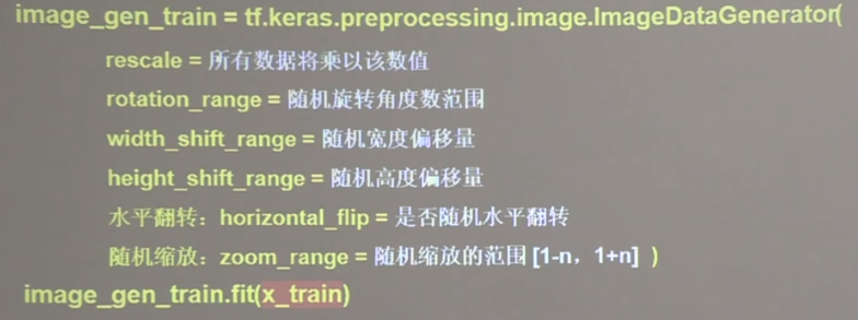
数据增强 可用作增大数据量
fit fit(x, augment=False, rounds=1, seed=None)
将数据生成器用于某些样本数据数据。它基于一组样本数据,计算与数据转换相关的内部数据统计。当且仅当 featurewise_center 或 featurewise_std_normalization 或 zca_whitening 设置为 True 时才需要。
x : 样本数据。秩应该为 4,即(batch,width,height,channel)的格式。对于灰度数据,通道轴的值应该为 1;对于 RGB 数据,值应该为 3。augment : 布尔值(默认为 False)。是否使用随机样本扩张。rounds : 整数(默认为 1)。如果数据数据增强(augment=True),表明在数据上进行多少次增强。seed : 整数(默认 None)。随机种子。
flow flow(x, y=None, batch_size=32, shuffle=True, sample_weight=None, seed=None, save_to_dir=None, save_prefix='', save_format='png', subset=None)
采集数据和标签数组,生成批量增强数据。
x : 输入数据。秩为 4 的 Numpy 矩阵或元组。如果是元组,第一个元素应该包含图像,第二个元素是另一个 Numpy 数组或一列 Numpy 数组,它们不经过任何修改就传递给输出。可用于将模型杂项数据与图像一起输入。对于灰度数据,图像数组的通道轴的值应该为 1,而对于 RGB 数据,其值应该为 3。y : 标签。batch_size : 整数 (默认为 32)。shuffle : 布尔值 (默认为 True)。sample_weight : 样本权重。seed : 整数(默认为 None)。save_to_dir : None 或 字符串(默认为 None)。这使您可以选择指定要保存的正在生成的增强图片的目录(用于可视化您正在执行的操作)。save_prefix : 字符串(默认 '')。保存图片的文件名前缀(仅当 save_to_dir 设置时可用)。save_format : “png”, “jpeg” 之一(仅当 save_to_dir 设置时可用)。默认:”png”。subset : 数据子集 (“training” 或 “validation”),如果 在 ImageDataGenerator 中设置了 validation_split。
返回一个生成元组 (x, y) 的 生成器Iterator,其中 x 是图像数据的 Numpy 数组(在单张图像输入时),或 Numpy 数组列表(在额外多个输入时),y 是对应的标签的 Numpy 数组。如果 ‘sample_weight’ 不是 None,生成的元组形式为 (x, y, sample_weight)。如果 y 是 None, 只有 Numpy 数组 x 被返回。
实现代码(部分) 1 2 3 4 5 6 7 8 9 10 11 12 13 14 15 from tensorflow.keras.preprocessing.image import ImageDataGeneratorx_train = x_train.reshape(x_train.shape[0 ], 28 , 28 , 1 ) image_gen_train = ImageDataGenerator( rescale=1. / 1. , rotation_range=45 , width_shift_range=.15 , height_shift_range=.15 , horizontal_flip=False , zoom_range=0.5 ) image_gen_train.fit(x_train) model.fit(image_gen_train.flow(x_train, y_train, batch_size=32 ), epochs=5 , validation_data=(x_test, y_test), validation_freq=1 )
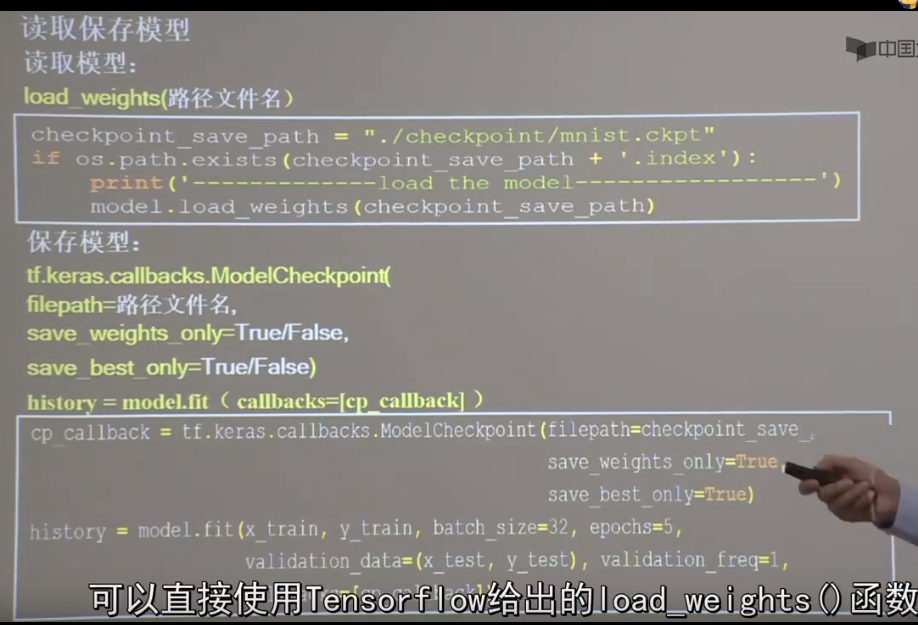
断点续训 将之前训练好的模型加载进来,在原来模型的基础上再进行训练
实现代码 1 2 3 4 5 6 7 8 9 10 11 12 13 14 15 16 17 18 19 20 21 22 23 24 25 26 27 28 29 import tensorflow as tfimport osmnist = tf.keras.datasets.mnist (x_train, y_train), (x_test, y_test) = mnist.load_data() x_train, x_test = x_train / 255.0 , x_test / 255.0 model = tf.keras.models.Sequential([ tf.keras.layers.Flatten(), tf.keras.layers.Dense(128 , activation='relu' ), tf.keras.layers.Dense(10 , activation='softmax' ) ]) model.compile(optimizer='adam' , loss=tf.keras.losses.SparseCategoricalCrossentropy(from_logits=False ), metrics=['sparse_categorical_accuracy' ]) checkpoint_save_path = "./checkpoint/mnist.ckpt" if os.path.exists(checkpoint_save_path + '.index' ): print('-------------load the model-----------------' ) model.load_weights(checkpoint_save_path) cp_callback = tf.keras.callbacks.ModelCheckpoint(filepath=checkpoint_save_path, save_weights_only=True , save_best_only=True ) history = model.fit(x_train, y_train, batch_size=32 , epochs=5 , validation_data=(x_test, y_test), validation_freq=1 , callbacks=[cp_callback]) model.summary()
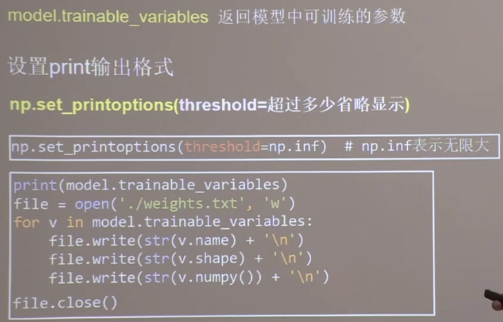
参数提取
实现代码(部分) 1 2 3 4 5 6 7 8 9 10 import numpy as npnp.set_printoptions(threshold=np.inf) print(model.trainable_variables) file = open('./weights.txt' , 'w' ) for v in model.trainable_variables: file.write(str(v.name) + '\n' ) file.write(str(v.shape) + '\n' ) file.write(str(v.numpy()) + '\n' ) file.close()
acc/loss可视化 加入绘图模块
实现代码(部分)
1 2 3 4 5 6 7 8 9 10 11 12 13 14 15 16 17 18 19 20 21 22 23 from matplotlib import pyplot as plthistory = model.fit(x_train, y_train, batch_size=32 , epochs=5 , validation_data=(x_test, y_test), validation_freq=1 , callbacks=[cp_callback]) acc = history.history['sparse_categorical_accuracy' ] val_acc = history.history['val_sparse_categorical_accuracy' ] loss = history.history['loss' ] val_loss = history.history['val_loss' ] plt.subplot(1 , 2 , 1 ) plt.plot(acc, label='Training Accuracy' ) plt.plot(val_acc, label='Validation Accuracy' ) plt.title('Training and Validation Accuracy' ) plt.legend() plt.subplot(1 , 2 , 2 ) plt.plot(loss, label='Training Loss' ) plt.plot(val_loss, label='Validation Loss' ) plt.title('Training and Validation Loss' ) plt.legend() plt.show()
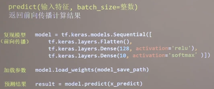
实现预测 在已训练好模型的基础上实现预测
实现代码(部分) 1 2 3 4 5 6 7 8 9 10 11 12 13 14 15 16 17 18 19 for i in range(preNum): image_path = input("the path of test picture:" ) img = Image.open(image_path) img = img.resize((28 , 28 ), Image.ANTIALIAS) img_arr = np.array(img.convert('L' )) for i in range(28 ): for j in range(28 ): if img_arr[i][j] < 200 : img_arr[i][j] = 255 else : img_arr[i][j] = 0 img_arr = img_arr / 255.0 x_predict = img_arr[tf.newaxis, ...] result = model.predict(x_predict) pred = tf.argmax(result, axis=1 ) print('\n' ) tf.print(pred)
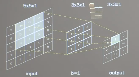
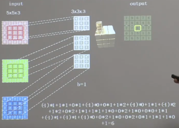
卷积神经网络 基本概念 卷积核 输出层对应特征为此时对应位置所有特征乘积之和
单通道卷积核
三通道卷积核
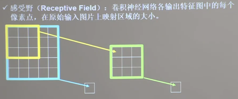
感受野 如图,黄色的卷积核感受野为3×3,绿色和蓝色卷积核的感受野为5×5
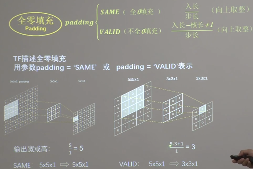
全零填充 在输入图的周围填充一层0
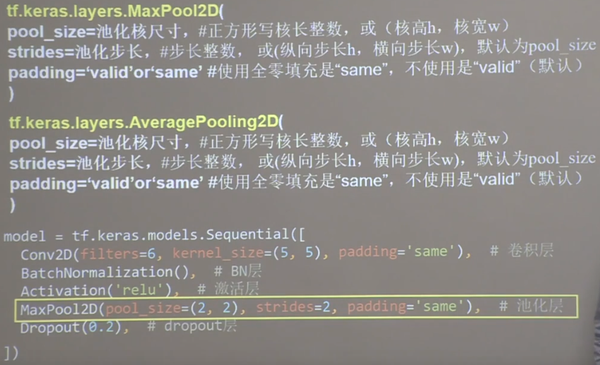
实现卷积层
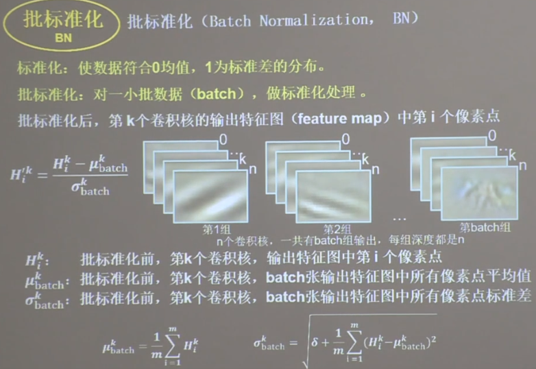
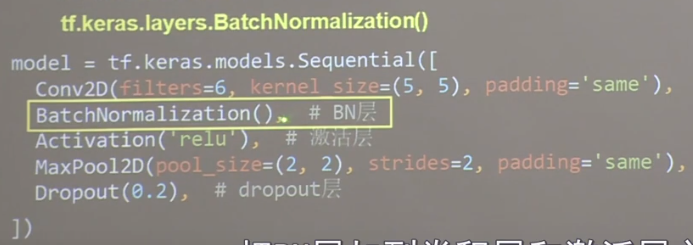
批标准化BN 位于卷积层之后,激活层之前
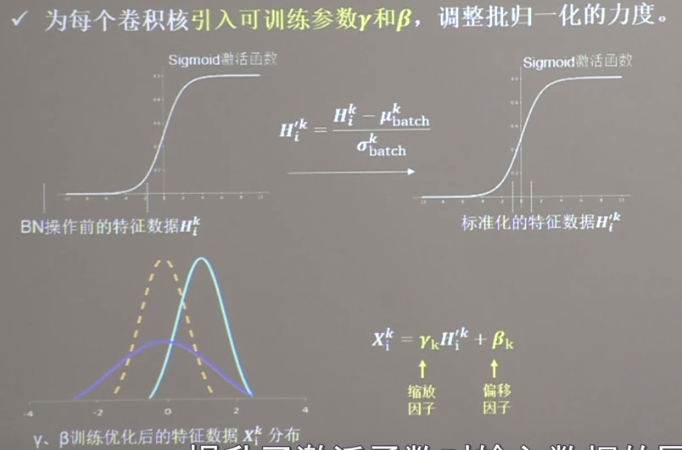
归一化提升了激活函数对输入数据的区分力,但会使得函数丧失非线性,可添加参数作以调整
tf实现
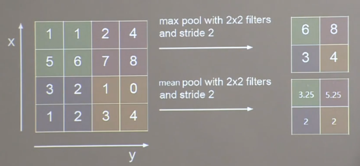
池化 减少卷积神经网络中特征数据量
最大池化提取图片纹理
均值池化保留背景特征
如图使用2×2的池化核对4×4图片进行操作,每次移动步长为2,得到不同的结果
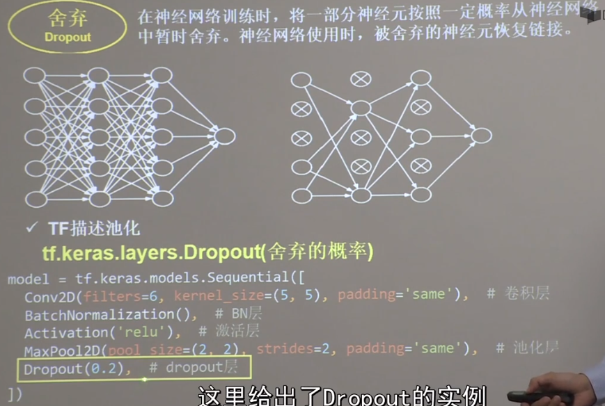
舍弃 训练时随机舍弃一部分神经元,防止过拟合,使用时回复神经元
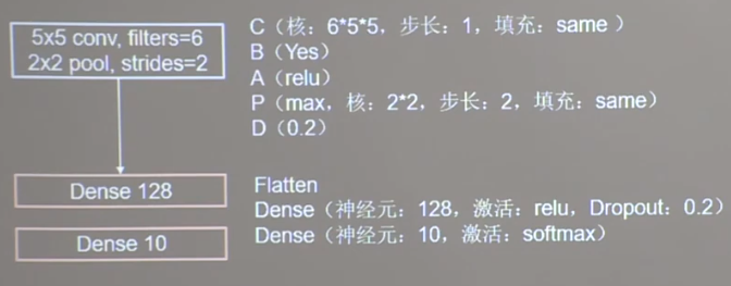
总体实现 过程:CBAPD
卷积核()
批标准化()
激活函数()
池化核()
舍弃()
自定义模型 之后的经典卷积网络都基于此代码
1 2 3 4 5 6 7 8 9 10 11 12 13 14 15 16 17 18 19 20 21 22 23 24 25 26 class Baseline (Model ): def __init__ (self ): super(Baseline, self).__init__() self.c1 = Conv2D(filters=6 , kernel_size=(5 , 5 ), padding='same' ) self.b1 = BatchNormalization() self.a1 = Activation('relu' ) self.p1 = MaxPool2D(pool_size=(2 , 2 ), strides=2 , padding='same' ) self.d1 = Dropout(0.2 ) self.flatten = Flatten() self.f1 = Dense(128 , activation='relu' ) self.d2 = Dropout(0.2 ) self.f2 = Dense(10 , activation='softmax' ) def call (self, x ): x = self.c1(x) x = self.b1(x) x = self.a1(x) x = self.p1(x) x = self.d1(x) x = self.flatten(x) x = self.f1(x) x = self.d2(x) y = self.f2(x) return y
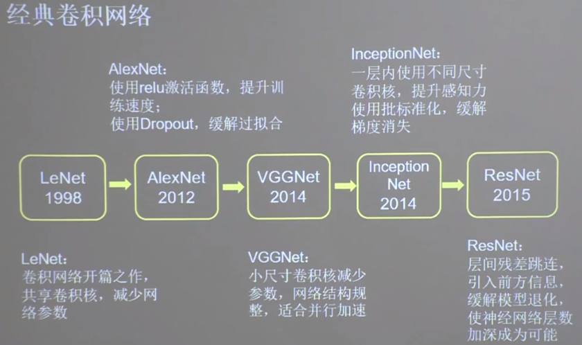
经典卷积网络
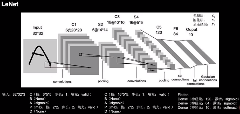
LeNet 共享卷积层减少网络的参数
(统计层数时只统计卷积计算层和全连接计算层)
共5层,2层卷积层,3层全连接层,一层Flatten层
模型代码 1 2 3 4 5 6 7 8 9 10 11 12 13 14 15 class LeNet5 (Model ): def __init__ (self ): super(LeNet5, self).__init__() self.c1 = Conv2D(filters=6 , kernel_size=(5 , 5 ), activation='sigmoid' ) self.p1 = MaxPool2D(pool_size=(2 , 2 ), strides=2 ) self.c2 = Conv2D(filters=16 , kernel_size=(5 , 5 ), activation='sigmoid' ) self.p2 = MaxPool2D(pool_size=(2 , 2 ), strides=2 ) self.flatten = Flatten() self.f1 = Dense(120 , activation='sigmoid' ) self.f2 = Dense(84 , activation='sigmoid' ) self.f3 = Dense(10 , activation='softmax' )
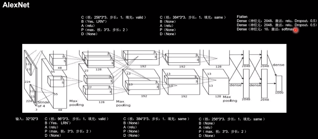
AlexNet 共8层,5层卷积层,3层全连接层,一层Flatten层
注:LRN近年来使用较少,效果与BN类似,故使用BN作为替代
模型代码 1 2 3 4 5 6 7 8 9 10 11 12 13 14 15 16 17 18 19 20 21 22 23 24 25 26 27 28 29 class AlexNet8 (Model ): def __init__ (self ): super(AlexNet8, self).__init__() self.c1 = Conv2D(filters=96 , kernel_size=(3 , 3 )) self.b1 = BatchNormalization() self.a1 = Activation('relu' ) self.p1 = MaxPool2D(pool_size=(3 , 3 ), strides=2 ) self.c2 = Conv2D(filters=256 , kernel_size=(3 , 3 )) self.b2 = BatchNormalization() self.a2 = Activation('relu' ) self.p2 = MaxPool2D(pool_size=(3 , 3 ), strides=2 ) self.c3 = Conv2D(filters=384 , kernel_size=(3 , 3 ), padding='same' , activation='relu' ) self.c4 = Conv2D(filters=384 , kernel_size=(3 , 3 ), padding='same' , activation='relu' ) self.c5 = Conv2D(filters=256 , kernel_size=(3 , 3 ), padding='same' , activation='relu' ) self.p3 = MaxPool2D(pool_size=(3 , 3 ), strides=2 ) self.flatten = Flatten() self.f1 = Dense(2048 , activation='relu' ) self.d1 = Dropout(0.5 ) self.f2 = Dense(2048 , activation='relu' ) self.d2 = Dropout(0.5 ) self.f3 = Dense(10 , activation='softmax' )
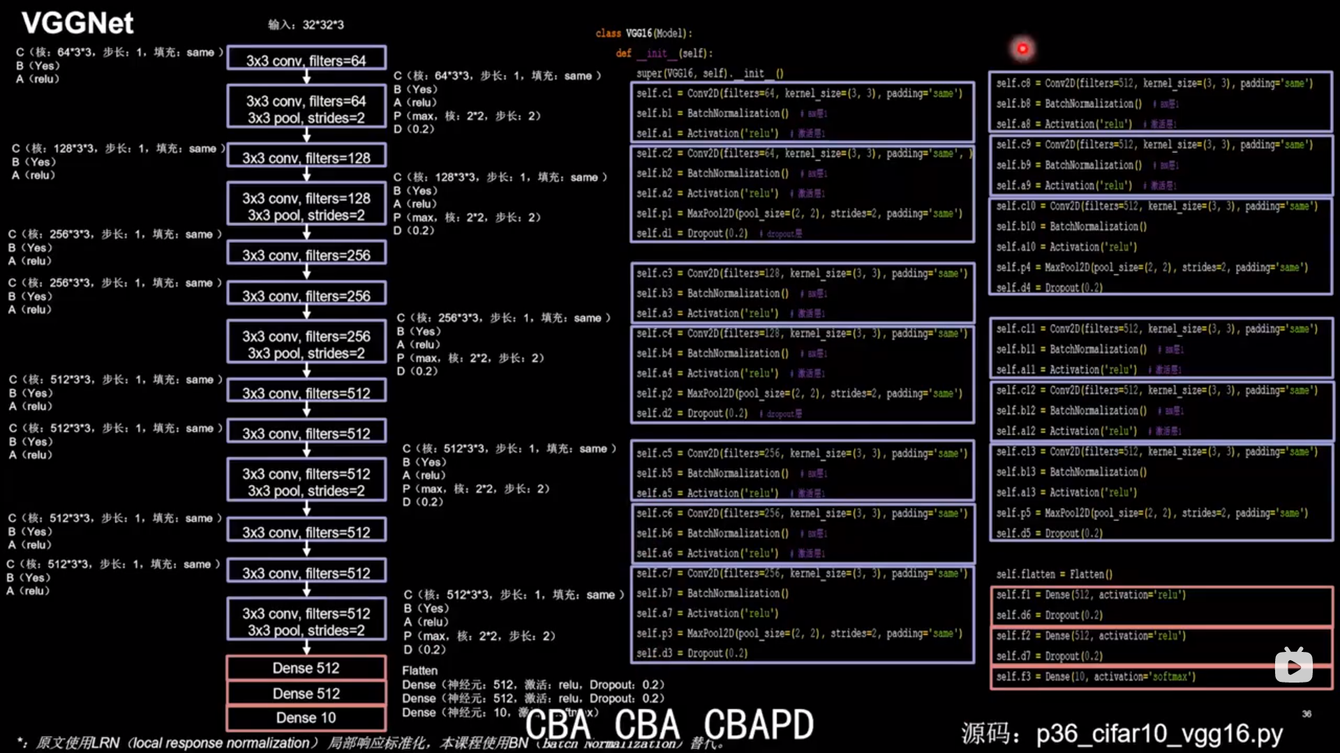
VGGNet 使用小尺寸卷积核,减少参数的同时提高了识别准确率,网络结构规整,适合硬件加速
在CBAPD的卷积层之间加入CBA的卷积层
16层VGGNet实例
1 2 3 4 5 6 7 8 9 10 11 12 13 14 15 16 17 18 19 20 21 22 23 24 25 26 27 28 29 30 31 32 33 34 35 36 37 38 39 40 41 42 43 44 45 46 47 48 49 50 51 52 53 54 55 56 57 58 59 60 61 62 63 class VGG16 (Model ): def __init__ (self ): super(VGG16, self).__init__() self.c1 = Conv2D(filters=64 , kernel_size=(3 , 3 ), padding='same' ) self.b1 = BatchNormalization() self.a1 = Activation('relu' ) self.c2 = Conv2D(filters=64 , kernel_size=(3 , 3 ), padding='same' , ) self.b2 = BatchNormalization() self.a2 = Activation('relu' ) self.p1 = MaxPool2D(pool_size=(2 , 2 ), strides=2 , padding='same' ) self.d1 = Dropout(0.2 ) self.c3 = Conv2D(filters=128 , kernel_size=(3 , 3 ), padding='same' ) self.b3 = BatchNormalization() self.a3 = Activation('relu' ) self.c4 = Conv2D(filters=128 , kernel_size=(3 , 3 ), padding='same' ) self.b4 = BatchNormalization() self.a4 = Activation('relu' ) self.p2 = MaxPool2D(pool_size=(2 , 2 ), strides=2 , padding='same' ) self.d2 = Dropout(0.2 ) self.c5 = Conv2D(filters=256 , kernel_size=(3 , 3 ), padding='same' ) self.b5 = BatchNormalization() self.a5 = Activation('relu' ) self.c6 = Conv2D(filters=256 , kernel_size=(3 , 3 ), padding='same' ) self.b6 = BatchNormalization() self.a6 = Activation('relu' ) self.c7 = Conv2D(filters=256 , kernel_size=(3 , 3 ), padding='same' ) self.b7 = BatchNormalization() self.a7 = Activation('relu' ) self.p3 = MaxPool2D(pool_size=(2 , 2 ), strides=2 , padding='same' ) self.d3 = Dropout(0.2 ) self.c8 = Conv2D(filters=512 , kernel_size=(3 , 3 ), padding='same' ) self.b8 = BatchNormalization() self.a8 = Activation('relu' ) self.c9 = Conv2D(filters=512 , kernel_size=(3 , 3 ), padding='same' ) self.b9 = BatchNormalization() self.a9 = Activation('relu' ) self.c10 = Conv2D(filters=512 , kernel_size=(3 , 3 ), padding='same' ) self.b10 = BatchNormalization() self.a10 = Activation('relu' ) self.p4 = MaxPool2D(pool_size=(2 , 2 ), strides=2 , padding='same' ) self.d4 = Dropout(0.2 ) self.c11 = Conv2D(filters=512 , kernel_size=(3 , 3 ), padding='same' ) self.b11 = BatchNormalization() self.a11 = Activation('relu' ) self.c12 = Conv2D(filters=512 , kernel_size=(3 , 3 ), padding='same' ) self.b12 = BatchNormalization() self.a12 = Activation('relu' ) self.c13 = Conv2D(filters=512 , kernel_size=(3 , 3 ), padding='same' ) self.b13 = BatchNormalization() self.a13 = Activation('relu' ) self.p5 = MaxPool2D(pool_size=(2 , 2 ), strides=2 , padding='same' ) self.d5 = Dropout(0.2 ) self.flatten = Flatten() self.f1 = Dense(512 , activation='relu' ) self.d6 = Dropout(0.2 ) self.f2 = Dense(512 , activation='relu' ) self.d7 = Dropout(0.2 ) self.f3 = Dense(10 , activation='softmax' )
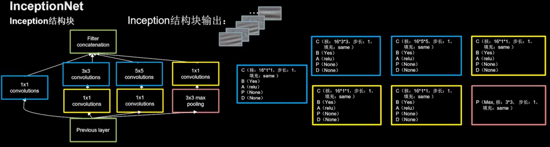
InceptionNet 同一层网络中使用不同尺寸的卷积核,提升模型感知力
精简版模型代码 1 2 3 4 5 6 7 8 9 10 11 12 13 14 15 16 17 18 19 20 21 22 23 24 25 26 27 28 29 30 31 32 33 34 35 36 37 38 39 40 41 42 43 44 45 46 47 48 49 50 51 52 53 54 55 56 57 58 59 60 61 62 63 64 65 66 67 class ConvBNRelu (Model ): def __init__ (self, ch, kernelsz=3 , strides=1 , padding='same' ): super(ConvBNRelu, self).__init__() self.model = tf.keras.models.Sequential([ Conv2D(ch, kernelsz, strides=strides, padding=padding), BatchNormalization(), Activation('relu' ) ]) def call (self, x ): x = self.model(x, training=False ) return x class InceptionBlk (Model ): def __init__ (self, ch, strides=1 ): super(InceptionBlk, self).__init__() self.ch = ch self.strides = strides self.c1 = ConvBNRelu(ch, kernelsz=1 , strides=strides) self.c2_1 = ConvBNRelu(ch, kernelsz=1 , strides=strides) self.c2_2 = ConvBNRelu(ch, kernelsz=3 , strides=1 ) self.c3_1 = ConvBNRelu(ch, kernelsz=1 , strides=strides) self.c3_2 = ConvBNRelu(ch, kernelsz=5 , strides=1 ) self.p4_1 = MaxPool2D(3 , strides=1 , padding='same' ) self.c4_2 = ConvBNRelu(ch, kernelsz=1 , strides=strides) def call (self, x ): x1 = self.c1(x) x2_1 = self.c2_1(x) x2_2 = self.c2_2(x2_1) x3_1 = self.c3_1(x) x3_2 = self.c3_2(x3_1) x4_1 = self.p4_1(x) x4_2 = self.c4_2(x4_1) x = tf.concat([x1, x2_2, x3_2, x4_2], axis=3 ) return x class Inception10 (Model ): def __init__ (self, num_blocks, num_classes, init_ch=16 , **kwargs ): super(Inception10, self).__init__(**kwargs) self.in_channels = init_ch self.out_channels = init_ch self.num_blocks = num_blocks self.init_ch = init_ch self.c1 = ConvBNRelu(init_ch) self.blocks = tf.keras.models.Sequential() for block_id in range(num_blocks): for layer_id in range(2 ): if layer_id == 0 : block = InceptionBlk(self.out_channels, strides=2 ) else : block = InceptionBlk(self.out_channels, strides=1 ) self.blocks.add(block) self.out_channels *= 2 self.p1 = GlobalAveragePooling2D() self.f1 = Dense(num_classes, activation='softmax' ) def call (self, x ): x = self.c1(x) x = self.blocks(x) x = self.p1(x) y = self.f1(x) return y
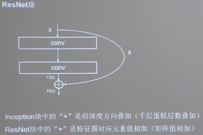
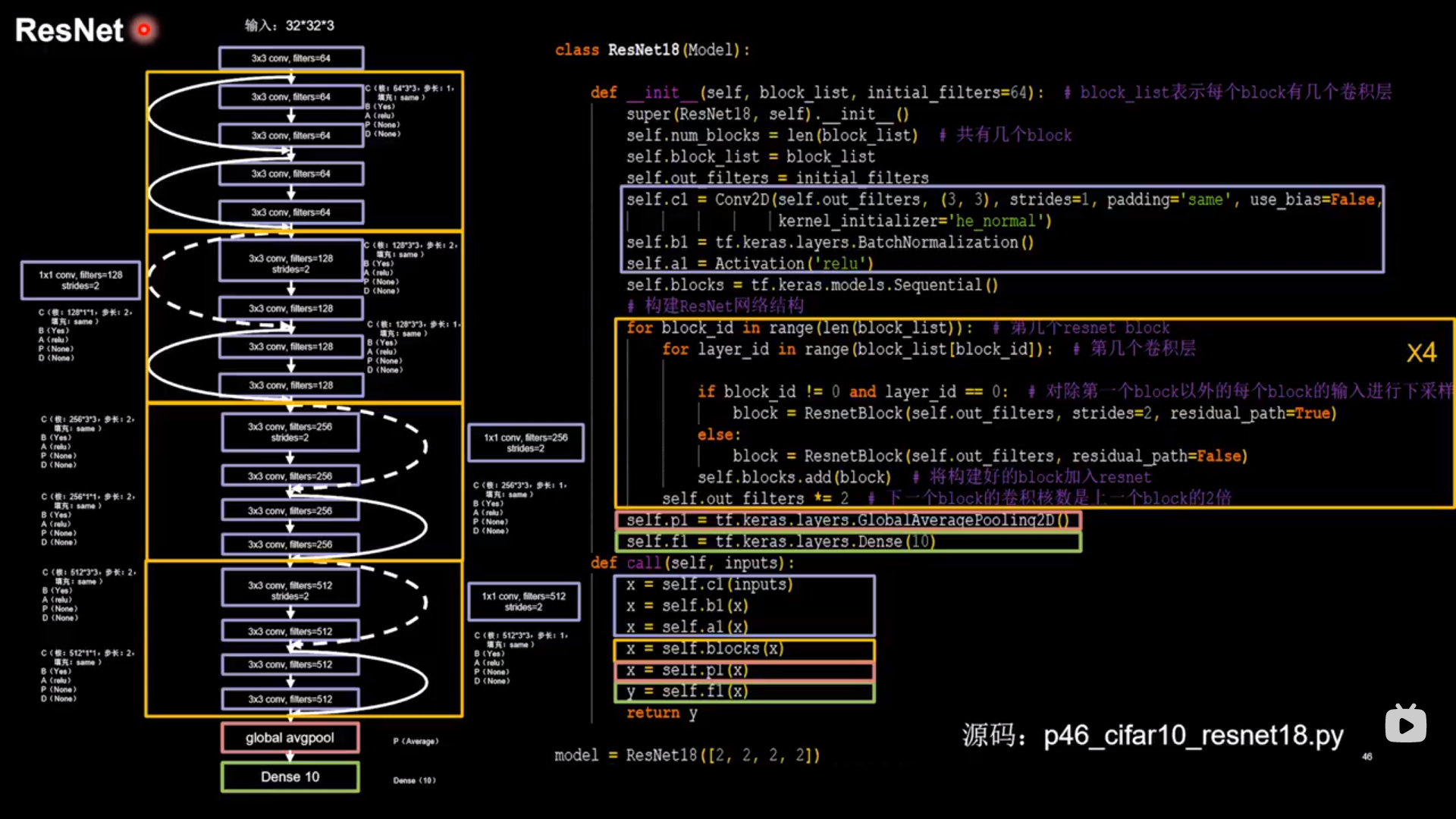
ResNet 应用层间残差跳连,缓解梯度消失
模型代码 1 2 3 4 5 6 7 8 9 10 11 12 13 14 15 16 17 18 19 20 21 class ResnetBlock (Model ): def __init__ (self, filters, strides=1 , residual_path=False ): super(ResnetBlock, self).__init__() self.filters = filters self.strides = strides self.residual_path = residual_path self.c1 = Conv2D(filters, (3 , 3 ), strides=strides, padding='same' , use_bias=False ) self.b1 = BatchNormalization() self.a1 = Activation('relu' ) self.c2 = Conv2D(filters, (3 , 3 ), strides=1 , padding='same' , use_bias=False ) self.b2 = BatchNormalization() if residual_path: self.down_c1 = Conv2D(filters, (1 , 1 ), strides=strides, padding='same' , use_bias=False ) self.down_b1 = BatchNormalization() self.a2 = Activation('relu' )
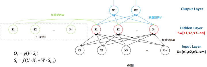
循环神经网络 实现短期记忆
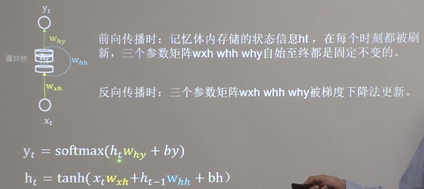
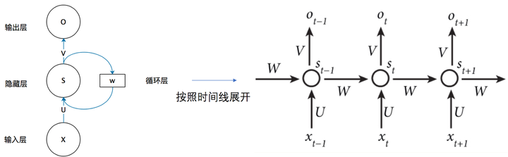
基本概念 循环核 具有’记忆力‘,通过不同时刻的参数共享实现对时间序列的信息提取
循环核时间步展开
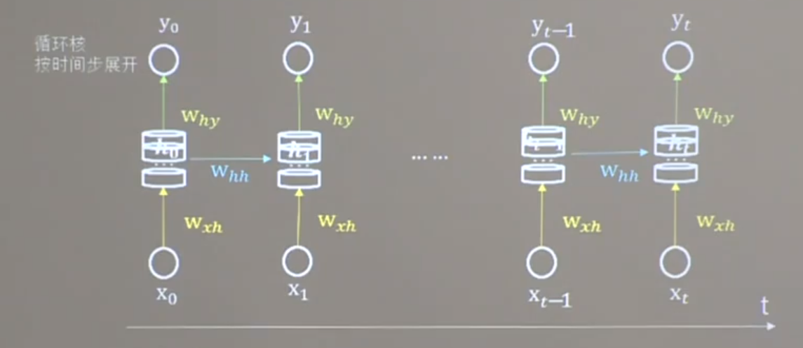
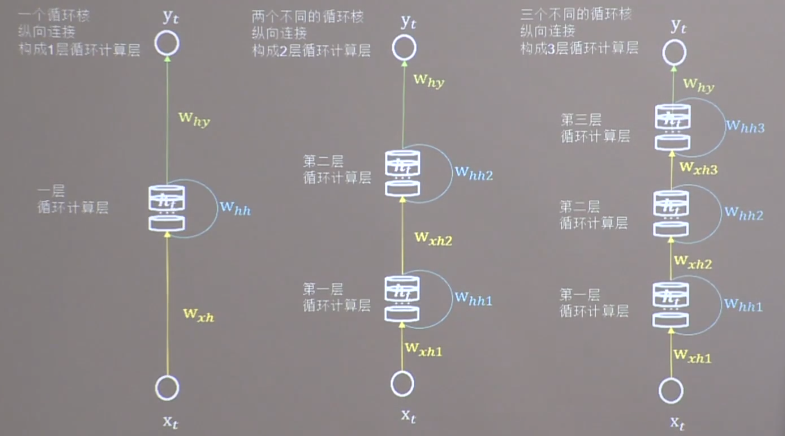
循环计算层 越靠近输出方向层数越高
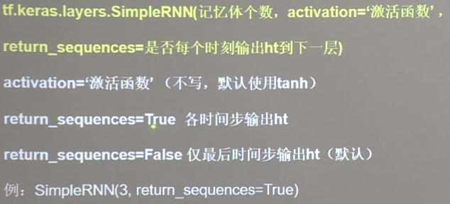
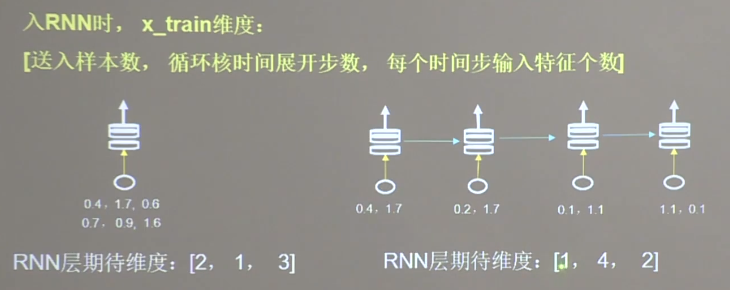
实现循环计算层
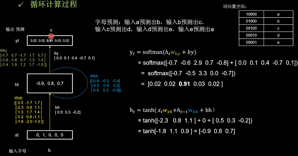
循环计算过程
one-hot实现预测字母 1 2 3 4 5 6 7 8 9 10 11 12 13 14 15 16 17 18 19 20 21 22 23 24 25 26 27 28 29 30 31 32 33 34 35 36 37 38 39 40 41 42 43 44 45 46 47 48 49 50 51 52 53 54 55 56 57 58 59 60 61 62 63 64 65 66 67 68 69 70 71 72 73 74 75 76 77 78 79 80 81 82 83 84 85 86 87 import numpy as npimport tensorflow as tffrom tensorflow.keras.layers import Dense, SimpleRNNimport matplotlib.pyplot as pltimport osinput_word = "abcde" w_to_id = {'a' : 0 , 'b' : 1 , 'c' : 2 , 'd' : 3 , 'e' : 4 } id_to_onehot = {0 : [1. , 0. , 0. , 0. , 0. ], 1 : [0. , 1. , 0. , 0. , 0. ], 2 : [0. , 0. , 1. , 0. , 0. ], 3 : [0. , 0. , 0. , 1. , 0. ], 4 : [0. , 0. , 0. , 0. , 1. ]} x_train = [id_to_onehot[w_to_id['a' ]], id_to_onehot[w_to_id['b' ]], id_to_onehot[w_to_id['c' ]], id_to_onehot[w_to_id['d' ]], id_to_onehot[w_to_id['e' ]]] y_train = [w_to_id['b' ], w_to_id['c' ], w_to_id['d' ], w_to_id['e' ], w_to_id['a' ]] np.random.seed(7 ) np.random.shuffle(x_train) np.random.seed(7 ) np.random.shuffle(y_train) tf.random.set_seed(7 ) x_train = np.reshape(x_train, (len(x_train), 1 , 5 )) y_train = np.array(y_train) model = tf.keras.Sequential([ SimpleRNN(3 ), Dense(5 , activation='softmax' ) ]) model.compile(optimizer=tf.keras.optimizers.Adam(0.01 ), loss=tf.keras.losses.SparseCategoricalCrossentropy(from_logits=False ), metrics=['sparse_categorical_accuracy' ]) checkpoint_save_path = "./checkpoint/rnn_onehot_1pre1.ckpt" if os.path.exists(checkpoint_save_path + '.index' ): print('-------------load the model-----------------' ) model.load_weights(checkpoint_save_path) cp_callback = tf.keras.callbacks.ModelCheckpoint(filepath=checkpoint_save_path, save_weights_only=True , save_best_only=True , monitor='loss' ) history = model.fit(x_train, y_train, batch_size=32 , epochs=100 , callbacks=[cp_callback]) model.summary() file = open('./weights.txt' , 'w' ) for v in model.trainable_variables: file.write(str(v.name) + '\n' ) file.write(str(v.shape) + '\n' ) file.write(str(v.numpy()) + '\n' ) file.close() acc = history.history['sparse_categorical_accuracy' ] loss = history.history['loss' ] plt.subplot(1 , 2 , 1 ) plt.plot(acc, label='Training Accuracy' ) plt.title('Training Accuracy' ) plt.legend() plt.subplot(1 , 2 , 2 ) plt.plot(loss, label='Training Loss' ) plt.title('Training Loss' ) plt.legend() plt.show() preNum = int(input("input the number of test alphabet:" )) for i in range(preNum): alphabet1 = input("input test alphabet:" ) alphabet = [id_to_onehot[w_to_id[alphabet1]]] alphabet = np.reshape(alphabet, (1 , 1 , 5 )) result = model.predict([alphabet]) pred = tf.argmax(result, axis=1 ) pred = int(pred) tf.print(alphabet1 + '->' + input_word[pred])
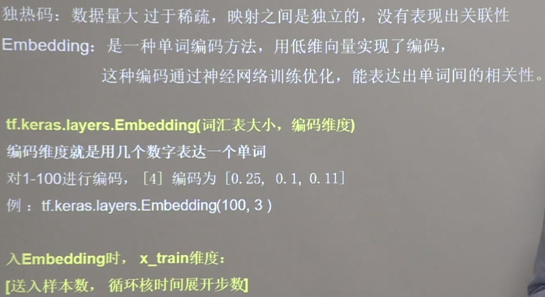
Embedding实现预测字母 用低维向量实现编码
1 2 3 4 5 6 7 8 9 10 11 12 13 14 15 16 17 18 19 20 21 22 23 24 25 26 27 28 29 30 31 32 33 34 35 36 37 38 39 40 41 42 43 44 45 46 47 48 49 50 51 52 53 54 55 56 57 58 59 60 61 62 63 64 65 66 67 68 69 70 71 72 73 74 75 76 77 78 79 80 81 82 83 84 85 86 import numpy as npimport tensorflow as tffrom tensorflow.keras.layers import Dense, SimpleRNN, Embeddingimport matplotlib.pyplot as pltimport osinput_word = "abcde" w_to_id = {'a' : 0 , 'b' : 1 , 'c' : 2 , 'd' : 3 , 'e' : 4 } x_train = [w_to_id['a' ], w_to_id['b' ], w_to_id['c' ], w_to_id['d' ], w_to_id['e' ]] y_train = [w_to_id['b' ], w_to_id['c' ], w_to_id['d' ], w_to_id['e' ], w_to_id['a' ]] np.random.seed(7 ) np.random.shuffle(x_train) np.random.seed(7 ) np.random.shuffle(y_train) tf.random.set_seed(7 ) x_train = np.reshape(x_train, (len(x_train), 1 )) y_train = np.array(y_train) model = tf.keras.Sequential([ Embedding(5 , 2 ), SimpleRNN(3 ), Dense(5 , activation='softmax' ) ]) model.compile(optimizer=tf.keras.optimizers.Adam(0.01 ), loss=tf.keras.losses.SparseCategoricalCrossentropy(from_logits=False ), metrics=['sparse_categorical_accuracy' ]) checkpoint_save_path = "./checkpoint/run_embedding_1pre1.ckpt" if os.path.exists(checkpoint_save_path + '.index' ): print('-------------load the model-----------------' ) model.load_weights(checkpoint_save_path) cp_callback = tf.keras.callbacks.ModelCheckpoint(filepath=checkpoint_save_path, save_weights_only=True , save_best_only=True , monitor='loss' ) history = model.fit(x_train, y_train, batch_size=32 , epochs=100 , callbacks=[cp_callback]) model.summary() file = open('./weights.txt' , 'w' ) for v in model.trainable_variables: file.write(str(v.name) + '\n' ) file.write(str(v.shape) + '\n' ) file.write(str(v.numpy()) + '\n' ) file.close() acc = history.history['sparse_categorical_accuracy' ] loss = history.history['loss' ] plt.subplot(1 , 2 , 1 ) plt.plot(acc, label='Training Accuracy' ) plt.title('Training Accuracy' ) plt.legend() plt.subplot(1 , 2 , 2 ) plt.plot(loss, label='Training Loss' ) plt.title('Training Loss' ) plt.legend() plt.show() preNum = int(input("input the number of test alphabet:" )) for i in range(preNum): alphabet1 = input("input test alphabet:" ) alphabet = [w_to_id[alphabet1]] alphabet = np.reshape(alphabet, (1 , 1 )) result = model.predict(alphabet) pred = tf.argmax(result, axis=1 ) pred = int(pred) tf.print(alphabet1 + '->' + input_word[pred])
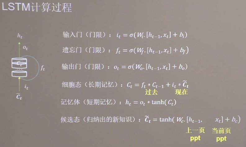
长短记忆网络(LSTM)
实现方法
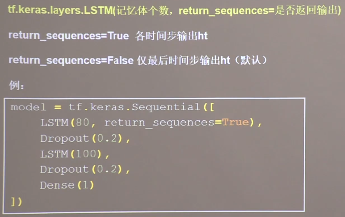
实现代码(部分) 1 2 3 4 5 6 7 8 9 from tensorflow.keras.layers import Dropout, Dense, LSTMmodel = tf.keras.Sequential([ LSTM(80 , return_sequences=True ), Dropout(0.2 ), LSTM(100 ), Dropout(0.2 ), Dense(1 ) ])
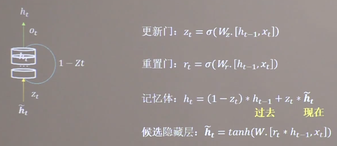
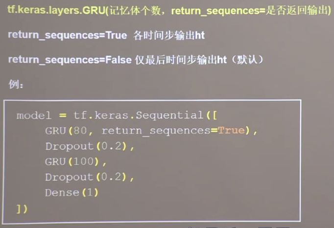
GRU网络 简化过后的LSTM网络,融合了长期记忆与短期记忆
计算过程
实现方法
实现代码(部分) 与LSTM相似
1 2 3 4 5 6 7 8 9 from tensorflow.keras.layers import Dropout, Dense, LSTMmodel = tf.keras.Sequential([ GRU(80 , return_sequences=True ), Dropout(0.2 ), GRU(100 ), Dropout(0.2 ), Dense(1 ) ])
其他神经网络 如深度置信神经网络DBN、生成对抗网络GAN等